Parametric Equations Of A Circle

Bear witness Mobile Notice Show All NotesHide All Notes

Mobile Notice

You lot appear to be on a device with a "narrow" screen width (i.e. you are probably on a mobile phone). Due to the nature of the mathematics on this site information technology is best views in landscape way. If your device is non in landscape mode many of the equations will run off the side of your device (should be able to gyre to see them) and some of the card items volition be cutting off due to the narrow screen width.

Section 3-1 : Parametric Equations and Curves

To this point (in both Calculus I and Calculus II) we've looked almost exclusively at functions in the form \(y = f\left( x \right)\) or \(10 = h\left( y \right)\) and almost all of the formulas that nosotros've developed crave that functions be in one of these ii forms. The problem is that not all curves or equations that we'd like to look at fall hands into this form.

Have, for example, a circle. Information technology is piece of cake plenty to write down the equation of a circumvolve centered at the origin with radius \(r\).

\[{x^ii} + {y^2} = {r^ii}\]

However, we will never exist able to write the equation of a circle downwardly equally a unmarried equation in either of the forms above. Sure we can solve for \(x\) or \(y\) as the post-obit ii formulas show

\[y = \pm \sqrt {{r^ii} - {x^ii}} \hspace{0.5in}\hspace{0.25in}ten = \pm \sqrt {{r^2} - {y^2}} \]

merely there are in fact ii functions in each of these. Each formula gives a portion of the circle.

\[\begin{marshal*}y & = \sqrt {{r^two} - {x^two}} & \hspace{0.15in} & \left( {{\mbox{acme}}} \correct) \hspace{0.75in}\ & ten & = \sqrt {{r^ii} - {y^2}} & \hspace{0.15in} & \left( {{\mbox{right side}}} \right)\\ y & = - \sqrt {{r^two} - {x^2}} & \hspace{0.15in} & \left( {{\mbox{bottom}}} \right)\hspace{0.75in} & ten & = - \sqrt {{r^two} - {y^ii}} & \hspace{0.15in} & \left( {{\mbox{left side}}} \right)\end{marshal*}\]

Unfortunately, we normally are working on the whole circumvolve, or simply tin can't say that we're going to exist working only on ane portion of information technology. Even if we can narrow things down to only one of these portions the function is still oftentimes adequately unpleasant to work with.

In that location are also a great many curves out at that place that we can't fifty-fifty write down every bit a single equation in terms of only \(10\) and \(y\). So, to deal with some of these problems we introduce parametric equations. Instead of defining \(y\) in terms of \(x\) (\(y = f\left( 10 \right)\)) or \(10\) in terms of \(y\) (\(10 = h\left( y \right)\)) nosotros ascertain both \(10\) and \(y\) in terms of a third variable called a parameter equally follows,

\[x = f\left( t \right)\hspace{0.5in}y = k\left( t \right)\]

This tertiary variable is usually denoted by \(t\) (as we did hither) merely doesn't have to exist of course. Sometimes nosotros volition restrict the values of \(t\) that we'll use and at other times we won't. This will often be dependent on the problem and just what we are attempting to do.

Each value of \(t\) defines a point \(\left( {x,y} \right) = \left( {f\left( t \right),thou\left( t \right)} \right)\) that we tin can plot. The drove of points that we get past letting \(t\) be all possible values is the graph of the parametric equations and is called the parametric curve.

To help visualize but what a parametric bend is pretend that we have a big tank of water that is in constant motility and we drib a ping pong ball into the tank. The point \(\left( {10,y} \right) = \left( {f\left( t \right),yard\left( t \right)} \correct)\) will then stand for the location of the ping pong ball in the tank at time \(t\) and the parametric curve will be a trace of all the locations of the ping pong brawl. Note that this is non ever a correct illustration but it is useful initially to help visualize only what a parametric curve is.

Sketching a parametric curve is non always an piece of cake affair to do. Let'south take a expect at an instance to come across 1 manner of sketching a parametric curve. This example will besides illustrate why this method is usually not the all-time.

Example ane Sketch the parametric curve for the following gear up of parametric equations. \[ten = {t^two} + t\hspace{0.5in}y = 2t - one\]

Evidence Solution

At this bespeak our merely option for sketching a parametric curve is to option values of \(t\), plug them into the parametric equations and then plot the points. So, permit'southward plug in some \(t\)'due south.

\(t\)	\(x\)	\(y\)
-two	ii	-5
-i	0	-iii
\( - \frac{1}{2}\)	\( - \frac{1}{4}\)	-2
0	0	-one
one	2	1

The outset question that should be asked at this point is, how did nosotros know to use the values of \(t\) that we did, especially the tertiary option? Unfortunately, at that place is no real answer to this question at this point. Nosotros simply selection \(t\)'s until we are adequately confident that we've got a adept thought of what the bend looks like. Information technology is this trouble with picking "expert" values of \(t\) that brand this method of sketching parametric curves 1 of the poorer choices. Sometimes nosotros have no selection, but if we do accept a option we should avoid it.

Nosotros'll talk over an alternate graphing method in later examples that will help to explicate how these values of \(t\) were chosen.

Nosotros have one more idea to discuss before we actually sketch the curve. Parametric curves take a direction of motion. The direction of motion is given by increasing \(t\). So, when plotting parametric curves, we likewise include arrows that show the direction of move. We will often requite the value of \(t\) that gave specific points on the graph also to make it clear the value of \(t\) that gave that item betoken.

Here is the sketch of this parametric curve.

Then, it looks similar we have a parabola that opens to the right.

Before we terminate this example in that location is a somewhat of import and subtle point that nosotros need to discuss first. Notice that we made certain to include a portion of the sketch to the correct of the points corresponding to \(t = - two\) and \(t = i\) to indicate that at that place are portions of the sketch there. Had we simply stopped the sketch at those points we are indicating that there was no portion of the curve to the correct of those points and there clearly will be. We just didn't compute any of those points.

This may seem similar an unimportant bespeak, only every bit nosotros'll see in the adjacent example it'southward more than important than we might recollect.

Earlier addressing a much easier style to sketch this graph permit'southward offset accost the issue of limits on the parameter. In the previous case we didn't have whatever limits on the parameter. Without limits on the parameter the graph volition continue in both directions as shown in the sketch above.

We will oft have limits on the parameter however and this will affect the sketch of the parametric equations. To come across this consequence let'southward look a slight variation of the previous case.

Case 2 Sketch the parametric bend for the post-obit set of parametric equations. \[x = {t^two} + t\hspace{0.5in}y = 2t - one\hspace{0.5in} - 1 \le t \le 1\]

Show Solution

Notation that the just difference here is the presence of the limits on \(t\). All these limits do is tell us that we can't have any value of \(t\) outside of this range. Therefore, the parametric curve will only be a portion of the curve above. Hither is the parametric curve for this example.

Notice that with this sketch we started and stopped the sketch right on the points originating from the end points of the range of \(t\)'due south. Dissimilarity this with the sketch in the previous example where we had a portion of the sketch to the right of the "start" and "end" points that nosotros computed.

In this instance the bend starts at \(t = - 1\) and ends at \(t = 1\), whereas in the previous example the curve didn't actually showtime at the right nigh points that we computed. We need to be clear in our sketches if the bend starts/ends correct at a point, or if that point was only the first/last one that we computed.

It is now time to take a expect at an easier method of sketching this parametric curve. This method uses the fact that in many, but not all, cases we tin actually eliminate the parameter from the parametric equations and get a function involving only \(x\) and \(y\). We volition sometimes phone call this the algebraic equation to differentiate it from the original parametric equations. There will be two small problems with this method, just it volition be like shooting fish in a barrel to accost those problems. It is important to note however that nosotros won't ever exist able to do this.

Just how we eliminate the parameter will depend upon the parametric equations that we've got. Permit's see how to eliminate the parameter for the set of parametric equations that nosotros've been working with to this point.

Example 3 Eliminate the parameter from the following fix of parametric equations. \[10 = {t^2} + t\hspace{0.5in}y = 2t - one\]

Bear witness Solution

One of the easiest ways to eliminate the parameter is to simply solve one of the equations for the parameter (\(t\), in this instance) and substitute that into the other equation. Note that while this may exist the easiest to eliminate the parameter, it'due south ordinarily non the all-time fashion as we'll meet soon enough.

In this case nosotros can easily solve \(y\) for \(t\).

\[t = \frac{one}{two}\left( {y + 1} \right)\]

Plugging this into the equation for \(x\) gives the following algebraic equation,

\[ten = {\left( {\frac{1}{2}\left( {y + 1} \right)} \right)^two} + \frac{one}{2}\left( {y + one} \correct) = \frac{1}{four}{y^ii} + y + \frac{iii}{4}\]

Sure enough from our Algebra noesis nosotros tin come across that this is a parabola that opens to the correct and volition have a vertex at \(\left( { - \frac{i}{iv}, - ii} \correct)\).

We won't carp with a sketch for this one equally we've already sketched this once and the bespeak here was more to eliminate the parameter anyway.

Earlier nosotros exit this example permit'due south address one quick issue.

In the first example we just, seemingly randomly, picked values of \(t\) to use in our tabular array, peculiarly the tertiary value. There really was no apparent reason for choosing \(t = - \frac{1}{2}\). It is even so probably the most important choice of \(t\) as it is the 1 that gives the vertex.

The reality is that when writing this material upwards we actually did this trouble offset then went dorsum and did the first problem. Plotting points is generally the way about people offset learn how to construct graphs and it does illustrate some important concepts, such as direction, so it made sense to do that beginning in the notes. In practice all the same, this example is often done first.

So, how did we become those values of \(t\)? Well permit's first off with the vertex as that is probably the most important point on the graph. We have the \(ten\) and \(y\) coordinates of the vertex and we also have \(x\) and \(y\) parametric equations for those coordinates. So, plug in the coordinates for the vertex into the parametric equations and solve for \(t\). Doing this gives,

\[\begin{array}{ll}{ - \frac{1}{iv} = {t^2} + t}\\{ - ii = 2t - 1}\stop{array}\hspace{0.5in} \Rightarrow \hspace{0.5in}\begin{array}{ll}{t = - \frac{1}{2}\,\,\,\left( {{\mbox{double root}}} \right)}\\{t = - \frac{1}{ii}}\terminate{array}\]

So, as we can see, the value of \(t\) that will give both of these coordinates is \(t = - \frac{1}{2}\). Notation that the \(10\) parametric equation gave a double root and this will often not happen. Often nosotros would accept gotten two distinct roots from that equation. In fact, it won't exist unusual to get multiple values of \(t\) from each of the equations.

Nonetheless, what we can say is that there will exist a value(s) of \(t\) that occurs in both sets of solutions and that is the \(t\) that we want for that point. We'll somewhen see an example where this happens in a later department.

Now, from this piece of work we tin see that if nosotros use \(t = - \frac{1}{2}\) nosotros volition get the vertex and and so we included that value of \(t\) in the table in Example 1. One time we had that value of \(t\) we chose 2 integer values of \(t\) on either side to finish out the table.

Every bit nosotros volition see in after examples in this section determining values of \(t\) that will give specific points is something that we'll need to practice on a fairly regular ground. It is adequately simple however equally this instance has shown. All we need to be able to do is solve a (usually) fairly basic equation which by this point in time shouldn't exist too difficult.

Getting a sketch of the parametric curve once we've eliminated the parameter seems fairly simple. All we need to do is graph the equation that we institute by eliminating the parameter. As noted already yet, there are 2 small problems with this method. The first is direction of motility. The equation involving just \(x\) and \(y\) will Non requite the direction of motion of the parametric curve. This is generally an easy trouble to gear up nevertheless. Let'southward take a quick await at the derivatives of the parametric equations from the final example. They are,

\[\begin{align*}\frac{{dx}}{{dt}} & = 2t + 1\\ \frac{{dy}}{{dt}} & = 2\cease{align*}\]

Now, all we demand to do is recall our Calculus I knowledge. The derivative of \(y\) with respect to \(t\) is clearly e'er positive. Recalling that one of the interpretations of the first derivative is rate of change nosotros now know that as \(t\) increases \(y\) must also increase. Therefore, nosotros must be moving up the curve from bottom to top as \(t\) increases as that is the only management that will always give an increasing \(y\) as \(t\) increases.

Note that the \(x\) derivative isn't as useful for this assay equally it will be both positive and negative and hence \(x\) volition exist both increasing and decreasing depending on the value of \(t\). That doesn't help with management much as following the curve in either direction will showroom both increasing and decreasing \(x\).

In some cases, merely one of the equations, such equally this example, will give the management while in other cases either ane could exist used. Information technology is besides possible that, in some cases, both derivatives would be needed to determine direction. It will always exist dependent on the private set of parametric equations.

The second problem with eliminating the parameter is all-time illustrated in an example as we'll be running into this problem in the remaining examples.

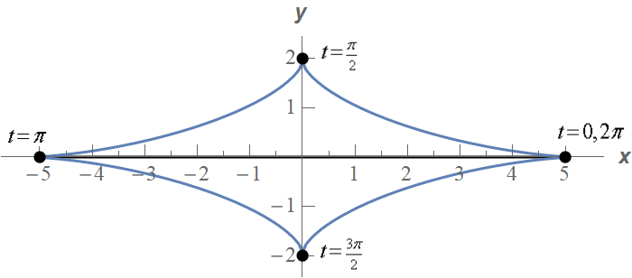
Instance 4 Sketch the parametric bend for the following ready of parametric equations. Clearly bespeak direction of motion. \[x = five\cos t\hspace{0.5in}y = two\sin t\hspace{0.5in}0 \le t \le ii\pi \]

Show Solution

Before we continue with eliminating the parameter for this problem permit's first address once again why only picking \(t\)'due south and plotting points is not really a good idea.

Given the range of \(t\)'south in the problem argument allow'south use the post-obit set of \(t\)'due south.

\(t\)	\(x\)	\(y\)
0	5	0
\(\frac{\pi }{2}\)	0	2
\(\pi \)	-5	0
\(\frac{{three\pi }}{2}\)	0	-ii
\(2\pi \)	five	0

The question that we need to ask now is do nosotros have plenty points to accurately sketch the graph of this prepare of parametric equations? Below are some sketches of some possible graphs of the parametric equation based merely on these v points.

Given the nature of sine/cosine you might be tempted to eliminate the diamond and the square just there is no denying that they are graphs that go through the given points. The get-go and third graphs both have some curvature to them then you might exist tempted to assume that i of those is the correct one given the sine/cosine in the equations. The last graph is as well a little empty-headed only it does show a graph going through the given points.

Again, given the nature of sine/cosine y'all are probably guessing that the correct graph is the the beginning or third graph. However, that is all that would be at this point. A estimate. Nothing really says unequivocally that the parametric bend is an volition be one of those two just from those 5 points. That is the danger of sketching parametric curves based on a handful of points. Unless we know what the graph will be ahead of time we are really just making a gauge.

It is important to annotation at this point that it is very easy to construct a set of parametric equations both containing sines and/or cosines and yet accept the graph not have whatever curvature at all. Yous can often make some guesses as to the shape of the curve from the parametric equations simply you won't ever guess correctly unfortunately. Intendance must exist taken when graphing parametric equations to non take the behavior of the individual parametric equations and just assume that behavior volition translate to the bend of the prepare of parametric equations.

Also, in full general, we should avoid plotting points to sketch parametric curves as that will, on occasion, lead to wrong graphs. The all-time method, provided information technology can be washed, is to eliminate the parameter. As noted simply prior to starting this example there is nevertheless a potential problem with eliminating the parameter that we'll need to deal with. We will eventually talk over this outcome. For now, let'south just proceed with eliminating the parameter.

We'll showtime past eliminating the parameter equally we did in the previous section. Nosotros'll solve i of the of the equations for \(t\) and plug this into the other equation. For instance, nosotros could do the following,

\[t = {\cos ^{ - 1}}\left( {\frac{ten}{v}} \correct)\hspace{0.5in} \Rightarrow \hspace{0.5in}y = 2\sin \left( {{{\cos }^{ - 1}}\left( {\frac{x}{five}} \right)} \right)\]

Can you see the problem with doing this? This is definitely like shooting fish in a barrel to do just we have a greater chance of correctly graphing the original parametric equations by plotting points than we practise graphing this!

There are many means to eliminate the parameter from the parametric equations and solving for \(t\) is commonly non the best mode to practise it. While information technology is oft like shooting fish in a barrel to do we will, in most cases, terminate upwards with an equation that is nigh impossible to bargain with.

So, how can we eliminate the parameter here? In this case all we demand to do is recall a very squeamish trig identity and the equation of an ellipse. Recall,

\[{\cos ^2}t + {\sin ^2}t = one\]

Then from the parametric equations we get,

\[\cos t = \frac{x}{5}\hspace{0.5in}\sin t = \frac{y}{two}\]

Then, using the trig identity from above and these equations we get,

\[ane = {\cos ^2}t + {\sin ^2}t = {\left( {\frac{x}{5}} \correct)^ii} + {\left( {\frac{y}{two}} \right)^2} = \frac{{{10^2}}}{{25}} + \frac{{{y^ii}}}{4}\]

Then we at present know that we will have an ellipse.

Now, allow's go along on with the example. We've identified that the parametric equations describe an ellipse, but we can't only sketch an ellipse and be washed with information technology.

Starting time, merely because the algebraic equation was an ellipse doesn't really hateful that the parametric bend is the total ellipse. It is always possible that the parametric bend is just a portion of the ellipse. In order to identify simply how much of the ellipse the parametric curve will cover permit's become back to the parametric equations and run across what they tell u.s. about any limits on \(x\) and \(y\). Based on our knowledge of sine and cosine we have the following,

\[\begin{align*} & - 1 \le \cos t \le 1\hspace{0.25in} \Rightarrow \hspace{0.25in} - five \le 5\cos t \le 5\hspace{0.25in} \Rightarrow \hspace{0.25in}\,\, - 5 \le ten \le five\\ & - 1 \le \sin t \le 1\hspace{0.25in} \Rightarrow \hspace{0.25in} - 2 \le 2\sin t \le 2 \,\hspace{0.25in} \Rightarrow \hspace{0.25in}\,\, - 2 \le y \le 2\stop{align*}\]

And so, by starting with sine/cosine and "building up" the equation for \(10\) and \(y\) using bones algebraic manipulations nosotros get that the parametric equations enforce the above limits on \(ten\) and \(y\). In this case, these also happen to be the full limits on \(x\) and \(y\) nosotros go by graphing the total ellipse.

This is the second potential result alluded to to a higher place. The parametric curve may not e'er trace out the full graph of the algebraic curve. We should e'er find limits on \(x\) and \(y\) enforced upon us by the parametric bend to make up one's mind just how much of the algebraic curve is really sketched out by the parametric equations.

Therefore, in this case, we now know that nosotros get a total ellipse from the parametric equations. Before we go on with the rest of the example be careful to non always just assume we volition get the full graph of the algebraic equation. At that place are definitely times when we will non go the full graph and we'll need to practice a similar analysis to determine merely how much of the graph we actually get. We'll meet an example of this later on.

Note too that whatsoever limits on \(t\) given in the problem statement tin also affect how much of the graph of the algebraic equation we get. In this instance nonetheless, based on the table of values we computed at the start of the trouble nosotros can see that nosotros practice indeed get the full ellipse in the range \(0 \le t \le 2\pi \). That won't always be the example however, then pay attention to whatever restrictions on \(t\) that might exist!

Next, we need to determine a direction of movement for the parametric bend. Think that all parametric curves have a direction of motion and the equation of the ellipse simply tells us zilch about the direction of movement.

To become the direction of movement it is tempting to simply utilise the table of values we computed in a higher place to get the direction of move. In this case, nosotros would judge (and aye that is all it is – a guess) that the curve traces out in a counter-clockwise direction. We'd be correct. In this example, we'd be correct! The problem is that tables of values can be misleading when determining a direction of motion as we'll see in the next example.

Therefore, information technology is best to non apply a table of values to determine the direction of motion. To correctly make up one's mind the direction of motion nosotros'll use the same method of determining the direction that we discussed after Example 3. In other words, we'll have the derivative of the parametric equations and utilize our knowledge of Calculus I and trig to make up one's mind the direction of motion.

The derivatives of the parametric equations are,

\[\frac{{dx}}{{dt}} = - 5\sin t\hspace{0.5in}\frac{{dy}}{{dt}} = 2\cos t\]

Now, at \(t = 0\) we are at the point \(\left( {5,0} \right)\) and let's see what happens if we starting time increasing \(t\). Allow'due south increase \(t\) from \(t = 0\) to \(t = \frac{\pi }{2}\). In this range of \(t\)'s nosotros know that sine is always positive and and then from the derivative of the \(x\) equation nosotros tin see that \(x\) must be decreasing in this range of \(t\)'southward.

This, however, doesn't actually help us decide a management for the parametric curve. Starting at \(\left( {5,0} \right)\) no affair if nosotros move in a clockwise or counter-clockwise direction \(x\) will have to decrease so we haven't actually learned annihilation from the \(x\) derivative.

The derivative from the \(y\) parametric equation on the other manus volition help united states of america. Once more, equally we increment \(t\) from \(t = 0\) to \(t = \frac{\pi }{2}\) we know that cosine will be positive and so \(y\) must exist increasing in this range. That notwithstanding, tin can simply happen if nosotros are moving in a counter‑clockwise direction. If nosotros were moving in a clockwise direction from the signal \(\left( {5,0} \right)\) we can encounter that \(y\) would take to subtract!

Therefore, in the first quadrant we must be moving in a counter-clockwise management. Allow's move on to the second quadrant.

So, we are now at the point \(\left( {0,2} \right)\) and we will increment \(t\) from \(t = \frac{\pi }{2}\) to \(t = \pi \). In this range of \(t\) we know that cosine will be negative and sine volition be positive. Therefore, from the derivatives of the parametric equations nosotros tin can meet that \(x\) is even so decreasing and \(y\) will now be decreasing every bit well.

In this quadrant the \(y\) derivative tells us nix as \(y\) only must decrease to move from \(\left( {0,ii} \right)\). However, in club for \(x\) to decrease, as we know information technology does in this quadrant, the direction must withal be moving a counter-clockwise rotation.

We are now at \(\left( { - 5,0} \correct)\) and we will increase \(t\) from \(t = \pi \) to \(t = \frac{{3\pi }}{ii}\). In this range of \(t\) we know that cosine is negative (and hence \(y\) will be decreasing) and sine is also negative (and hence \(ten\) volition exist increasing). Therefore, nosotros will continue to move in a counter‑clockwise movement.

For the 4^th quadrant nosotros will start at \(\left( {0, - ii} \right)\) and increase \(t\) from \(t = \frac{{iii\pi }}{ii}\) to \(t = 2\pi \). In this range of \(t\) nosotros know that cosine is positive (and hence \(y\) will be increasing) and sine is negative (and hence \(x\) will be increasing). So, as in the previous 3 quadrants, we go on to motility in a counter‑clockwise move.

At this point nosotros covered the range of \(t\)'s we were given in the problem argument and during the total range the move was in a counter-clockwise management.

Nosotros can now fully sketch the parametric curve and so, here is the sketch.

Okay, that was a actually long example. Most of these types of problems aren't as long. We just had a lot to discuss in this one and so we could get a couple of important ideas out of the way. The rest of the examples in this section shouldn't take as long to get through.

Now, let's have a look at another example that will illustrate an of import idea almost parametric equations.

Case 5 Sketch the parametric bend for the following set up of parametric equations. Clearly indicate direction of motion. \[x = 5\cos \left( {3t} \right)\hspace{0.5in}y = two\sin \left( {3t} \correct)\hspace{0.5in}0 \le t \le two\pi \]

Show Solution

Annotation that the only difference in betwixt these parametric equations and those in Example 4 is that nosotros replaced the \(t\) with 3\(t\). We can eliminate the parameter here in the same manner as nosotros did in the previous example.

\[\cos \left( {3t} \right) = \frac{x}{5}\hspace{0.5in}\sin \left( {3t} \right) = \frac{y}{2}\]

Nosotros and then get,

\[1 = {\cos ^2}\left( {3t} \right) + {\sin ^2}\left( {3t} \correct) = {\left( {\frac{x}{5}} \correct)^2} + {\left( {\frac{y}{ii}} \right)^2} = \frac{{{ten^ii}}}{{25}} + \frac{{{y^2}}}{4}\]

So, we get the same ellipse that we did in the previous instance. As well notation that we can practise the same analysis on the parametric equations to determine that nosotros take exactly the same limits on \(x\) and \(y\). Namely,

\[ - v \le x \le five\hspace{0.5in}\hspace{0.25in} - two \le y \le 2\]

Information technology'south starting to wait like irresolute the \(t\) into a 3\(t\) in the trig equations will not change the parametric bend in any style. That is not correct nevertheless. The curve does alter in a minor but important style which we volition be discussing soon.

Before discussing that small change the three\(t\) brings to the bend let's discuss the management of move for this curve. Despite the fact that nosotros said in the concluding instance that picking values of \(t\) and plugging in to the equations to find points to plot is a bad idea allow'south do it any mode.

Given the range of \(t\)'s from the problem argument the post-obit set looks like a skilful choice of \(t\)'s to use.

\(t\)	\(x\)	\(y\)
0	5	0
\(\frac{\pi }{2}\)	0	-2
\(\pi \)	-5	0
\(\frac{{3\pi }}{2}\)	0	2
\(2\pi \)	5	0

And then, the merely change to this table of values/points from the concluding example is all the nonzero \(y\) values changed sign. From a quick glance at the values in this table it would look similar the curve, in this case, is moving in a clockwise direction. But is that correct? Recall we said that these tables of values can be misleading when used to determine direction and that'southward why we don't employ them.

Let's see if our beginning impression is correct. Nosotros tin can check our commencement impression by doing the derivative piece of work to get the correct direction. Permit's work with just the \(y\) parametric equation as the \(x\) will have the aforementioned issue that it had in the previous example. The derivative of the \(y\) parametric equation is,

\[\frac{{dy}}{{dt}} = six\cos \left( {3t} \right)\]

Now, if we start at \(t = 0\) every bit nosotros did in the previous example and commencement increasing \(t\). At \(t = 0\) the derivative is clearly positive and and then increasing \(t\) (at to the lowest degree initially) will force \(y\) to besides be increasing. The but fashion for this to happen is if the bend is in fact tracing out in a counter-clockwise direction initially.

Now, we could go along to look at what happens equally nosotros farther increment \(t\), but when dealing with a parametric curve that is a full ellipse (equally this one is) and the statement of the trig functions is of the form nt for any constant \(due north\) the management will not change so one time we know the initial management we know that it will always move in that direction. Notation that this is only truthful for parametric equations in the course that we take here. Nosotros'll see in afterwards examples that for different kinds of parametric equations this may no longer be true.

Okay, from this analysis nosotros can meet that the curve must be traced out in a counter‑clockwise direction. This is direct counter to our guess from the tables of values to a higher place and so we can run across that, in this case, the table would probably have led us to the wrong direction. So, in one case once again, tables are generally not very reliable for getting pretty much any real information about a parametric curve other than a few points that must exist on the curve. Outside of that the tables are rarely useful and will by and large not be dealt with in further examples.

So, why did our table give an incorrect impression about the direction? Well call up that we mentioned earlier that the 3\(t\) volition atomic number 82 to a small only important change to the curve versus just a \(t\)? Allow's take a wait at just what that change is every bit information technology will besides answer what "went wrong" with our table of values.

Let's start past looking at \(t = 0\). At \(t = 0\) we are at the indicate \(\left( {5,0} \right)\) and let's ask ourselves what values of \(t\) put united states of america back at this point. We saw in Example 3 how to determine value(s) of \(t\) that put u.s.a. at certain points and the same procedure will work hither with a minor modification.

Instead of looking at both the \(x\) and \(y\) equations every bit we did in that example let's just look at the \(x\) equation. The reason for this is that we'll annotation that there are two points on the ellipse that volition have a \(y\) coordinate of zero, \(\left( {5,0} \right)\) and \(\left( { - 5,0} \right)\). If we gear up the \(y\) coordinate equal to naught we'll detect all the \(t\)'south that are at both of these points when nosotros only want the values of \(t\) that are at \(\left( {v,0} \correct)\).

So, because the \(x\) coordinate of five will only occur at this point nosotros tin simply use the \(x\) parametric equation to determine the values of \(t\) that will put usa at this betoken. Doing this gives the following equation and solution,

\[\begin{marshal*}5 & = v\cos \left( {3t} \correct)\,\\ 3t & = {\cos ^{ - i}}\left( 1 \right) = 0 + two\pi n\hspace{0.25in}\,\,\, \to \hspace{0.25in}\,\,\,\,\,\,t = \frac{2}{3}\pi n\,\,\,\,\,\,n = 0, \pm 1, \pm 2, \pm 3, \ldots \stop{align*}\]

Don't forget that when solving a trig equation nosotros need to add together on the "\( + 2\pi north\)" where \(n\) represents the number of total revolutions in the counter-clockwise direction (positive \(north\)) and clockwise management (negative \(due north\)) that we rotate from the get-go solution to get all possible solutions to the equation.

Now, let'southward plug in a few values of \(north\) starting at \(northward = 0\). We don't need negative \(n\) in this case since all of those would issue in negative \(t\) and those fall outside of the range of \(t\)'s nosotros were given in the problem argument. The first few values of \(t\) are then,

\[\brainstorm{align*}n & = 0\hspace{0.25in} : \hspace{0.25in} t = 0\\ northward & = 1\hspace{0.25in}:\hspace{0.25in}t = \frac{{2\pi }}{iii}\\ n & = 2\hspace{0.25in}:\hspace{0.25in}t = \frac{{four\pi }}{3}\\ n & = three\hspace{0.25in}:\hspace{0.25in}t = \frac{{half dozen\pi }}{3} = 2\pi \cease{align*}\]

Nosotros can stop here as all further values of \(t\) volition be outside the range of \(t\)'s given in this problem.

So, what is this telling us? Well dorsum in Instance 4 when the argument was just \(t\) the ellipse was traced out exactly in one case in the range \(0 \le t \le 2\pi \). However, when we change the argument to 3\(t\) (and recalling that the curve will always be traced out in a counter‑clockwise direction for this problem) we are going through the "starting" point of \(\left( {5,0} \right)\) ii more than times than nosotros did in the previous instance.

In fact, this bend is tracing out iii carve up times. The first trace is completed in the range \(0 \le t \le \frac{{2\pi }}{three}\). The second trace is completed in the range \(\frac{{2\pi }}{3} \le t \le \frac{{4\pi }}{3}\) and the third and final trace is completed in the range \(\frac{{4\pi }}{3} \le t \le two\pi \). In other words, irresolute the argument from \(t\) to 3\(t\) increase the speed of the trace and the curve will now trace out three times in the range \(0 \le t \le 2\pi \)!

This is why the table gives the wrong impression. The speed of the tracing has increased leading to an incorrect impression from the points in the table. The table seems to propose that betwixt each pair of values of \(t\) a quarter of the ellipse is traced out in the clockwise direction when in reality it is tracing out three quarters of the ellipse in the counter-clockwise direction.

Here's a concluding sketch of the bend and note that it really isn't all that different from the previous sketch. The simply differences are the values of \(t\) and the diverse points nosotros included. We did include a few more values of \(t\) at various points just to illustrate where the curve is at for diverse values of \(t\) but in general these really aren't needed.

So, we saw in the concluding two examples two sets of parametric equations that in some fashion gave the same graph. Yet, because they traced out the graph a different number of times we really practice need to think of them as different parametric curves at least in some manner. This may seem like a difference that nosotros don't demand to worry about, just equally nosotros will meet in later sections this can be a very important difference. In some of the later sections we are going to need a curve that is traced out exactly once.

Before we move on to other bug allow'south briefly acknowledge what happens past changing the \(t\) to an nt in these kinds of parametric equations. When nosotros are dealing with parametric equations involving but sines and cosines and they both take the aforementioned argument if nosotros modify the argument from \(t\) to nt we merely alter the speed with which the curve is traced out. If \(n > one\) we volition increase the speed and if \(n < 1\) we will decrease the speed.

Let's have a look at a couple more examples.

Example 6 Sketch the parametric curve for the following ready of parametric equations. Clearly identify the direction of motion. If the curve is traced out more than than one time give a range of the parameter for which the curve will trace out exactly once. \[10 = {\sin ^2}t\hspace{0.5in}y = 2\cos t\]

Testify Solution

We can eliminate the parameter much as we did in the previous two examples. Yet, nosotros'll need to annotation that the \(x\) already contains a \({\sin ^two}t\) and so we won't need to square the \(x\). We will nonetheless, need to square the \(y\) as we demand in the previous two examples.

\[10 + \frac{{{y^2}}}{four} = {\sin ^2}t + {\cos ^ii}t = ane\hspace{0.5in} \Rightarrow \hspace{0.5in}x = 1 - \frac{{{y^2}}}{4}\]

In this example the algebraic equation is a parabola that opens to the left.

We will need to exist very, very careful however in sketching this parametric curve. We will NOT go the whole parabola. A sketch of the algebraic form parabola volition exist for all possible values of \(y\). However, the parametric equations have defined both \(x\) and \(y\) in terms of sine and cosine and we know that the ranges of these are limited and and so nosotros won't get all possible values of \(x\) and \(y\) here. So, first let'south go limits on \(10\) and \(y\) as we did in previous examples. Doing this gives,

\[\begin{array}{ccccc} - ane \le \sin t \le 1 & \hspace{0.25in}\Rightarrow \hspace{0.25in} & 0 \le {\sin ^two}t \le one & \hspace{0.25in} \Rightarrow \hspace{0.25in} & 0 \le x \le 1\\ - one \le \cos t \le 1 & \hspace{0.25in} \Rightarrow \hspace{0.25in} & - ii \le two\cos t \le ii & \hspace{0.25in} \Rightarrow \hspace{0.25in} & - 2 \le y \le 2\end{assortment}\]

And so, it is clear from this that we will merely get a portion of the parabola that is defined past the algebraic equation. Below is a quick sketch of the portion of the parabola that the parametric curve will cover.

To cease the sketch of the parametric curve nosotros too demand the direction of motility for the bend. Before we get to that even so, let's jump frontwards and make up one's mind the range of \(t\)'s for one trace. To practice this we'll need to know the \(t\)'s that put united states at each end indicate and we can follow the same procedure we used in the previous case. The only difference is this time let's utilise the \(y\) parametric equation instead of the \(10\) because the \(y\) coordinates of the two end points of the curve are different whereas the \(ten\) coordinates are the aforementioned.

So, for the meridian signal we have,

\[\begin{align*}2 & = 2\cos t\\ t & = {\cos ^{ - 1}}\left( 1 \right) = 0 + 2\pi n = ii\pi due north,\hspace{0.25in}due north = 0, \pm ane, \pm 2, \pm 3, \ldots \terminate{align*}\]

For, plugging in some values of \(n\) we become that the curve will be at the peak point at,

\[t = \ldots , - 4\pi , - 2\pi ,0,2\pi ,4\pi , \ldots \]

Similarly, for the bottom point we have,

\[\begin{marshal*} - 2 & = 2\cos t\\ t & = {\cos ^{ - 1}}\left( { - 1} \right) = \pi + ii\pi northward,\hspace{0.25in}n = 0, \pm i, \pm two, \pm 3, \ldots \cease{align*}\]

So, we see that we will be at the bottom point at,

\[t = \ldots , - iii\pi , - \pi ,\pi ,3\pi , \ldots \]

And then, if we start at say, \(t = 0\), we are at the top point and we increase \(t\) nosotros have to move along the curve downwardly until nosotros reach \(t = \pi \) at which point we are now at the bottom betoken. This means that we will trace out the curve exactly in one case in the range \(0 \le t \le \pi \).

This is not the only range that will trace out the curve notwithstanding. Annotation that if nosotros farther increase \(t\) from \(t = \pi \) we will now take to travel back up the curve until nosotros accomplish \(t = 2\pi \) and we are at present back at the top bespeak. Increasing \(t\) again until we reach \(t = iii\pi \) will take u.s.a. dorsum down the curve until nosotros reach the bottom betoken again, etc. From this analysis nosotros tin can get two more ranges of \(t\) for 1 trace,

\[\pi \le t \le 2\pi \hspace{0.5in}2\pi \le t \le iii\pi \]

As you lot can probably see there are an infinite number of ranges of \(t\) we could use for one trace of the curve. Any of them would exist acceptable answers for this problem.

Note that in the process of determining a range of \(t\)'southward for one trace nosotros also managed to determine the direction of motion for this curve. In the range \(0 \le t \le \pi \) nosotros had to travel downwards along the curve to go from the top point at \(t = 0\) to the lesser point at \(t = \pi \). Notwithstanding, at \(t = 2\pi \) nosotros are back at the tiptop bespeak on the curve and to go there we must travel along the path. We can't just bound support to the top point or take a dissimilar path to get there. All travel must be done on the path sketched out. This ways that we had to get dorsum up the path. Further increasing \(t\) takes us back down the path, so upwardly the path once more etc.

In other words, this path is sketched out in both directions because we are not putting whatsoever restrictions on the \(t\)'s and then we take to assume nosotros are using all possible values of \(t\). If we had put restrictions on which \(t\)'s to use we might really have ended up only moving in one direction. That nonetheless would be a result only of the range of \(t\)'s we are using and not the parametric equations themselves.

Notation that nosotros didn't really need to do the above work to make up one's mind that the bend traces out in both directions.in this instance. Both the \(x\) and \(y\) parametric equations involve sine or cosine and we know both of those functions oscillate. This, in turn ways that both \(x\) and \(y\) volition oscillate as well. The only fashion for that to happen on this detail this curve will be for the curve to be traced out in both directions.

Be careful with the above reasoning that the oscillatory nature of sine/cosine forces the curve to be traced out in both directions. It tin can but be used in this instance because the "starting" point and "catastrophe" indicate of the curves are in different places. The only way to get from i of the "terminate" points on the curve to the other is to travel back along the curve in the reverse direction.

Contrast this with the ellipse in Example 4. In that case nosotros had sine/cosine in the parametric equations equally well. Yet, the curve only traced out in 1 direction, not in both directions. In Instance 4 we were graphing the full ellipse and then no matter where we offset sketching the graph nosotros will somewhen get back to the "starting" signal without ever retracing whatsoever portion of the graph. In Case four as we trace out the full ellipse both \(x\) and \(y\) do in fact oscillate between their ii "endpoints" only the bend itself does not trace out in both directions for this to happen.

Basically, we can only employ the oscillatory nature of sine/cosine to determine that the bend traces out in both directions if the curve starts and ends at dissimilar points. If the starting/ending bespeak is the aforementioned and so nosotros generally need to become through the full derivative statement to determine the actual direction of motion.

And so, to stop this problem out, below is a sketch of the parametric curve. Note that we put direction arrows in both directions to clearly indicate that it would exist traced out in both directions. We as well put in a few values of \(t\) just to help illustrate the direction of movement.

To this point nosotros've seen examples that would trace out the complete graph that we got by eliminating the parameter if we took a large enough range of \(t\)'s. Nonetheless, in the previous instance we've now seen that this volition not always be the case. It is more than possible to have a prepare of parametric equations which will continuously trace out just a portion of the curve. We can ordinarily decide if this volition happen by looking for limits on \(10\) and \(y\) that are imposed up us past the parametric equation.

We will often employ parametric equations to describe the path of an object or particle. Allow'south accept a look at an case of that.

Instance 7 The path of a particle is given by the following gear up of parametric equations. \[10 = iii\cos \left( {2t} \right)\hspace{0.5in}y = 1 + {\cos ^2}\left( {2t} \right)\]

Completely describe the path of this particle. Do this past sketching the path, determining limits on \(x\) and \(y\) and giving a range of \(t\)'southward for which the path will exist traced out exactly once (provide it traces out more than than once of course).

Show Solution

Eliminating the parameter this time will be a little different. We only have cosines this time and nosotros'll use that to our advantage. We can solve the \(x\) equation for cosine and plug that into the equation for \(y\). This gives,

\[\cos \left( {2t} \right) = \frac{x}{3}\hspace{0.5in}y = 1 + {\left( {\frac{ten}{three}} \right)^ii} = 1 + \frac{{{10^ii}}}{9}\]

This fourth dimension the algebraic equation is a parabola that opens upward. We also take the following limits on \(10\) and \(y\).

\[\begin{array}{ccccc} - 1 \le \cos \left( {2t} \right) \le 1 & \hspace{0.25in} & - 3 \le iii\cos \left( {2t} \right) \le 3 & \hspace{0.5in} & - three \le x \le 3\\ 0 \le {\cos ^ii}\left( {2t} \right) \le 1 & \hspace{0.25in} & ane \le one + {\cos ^two}\left( {2t} \right) \le two & \hspace{0.25in} & 1 \le y \le 2\stop{array}\]

So, again we only trace out a portion of the curve. Here is a quick sketch of the portion of the parabola that the parametric curve will cover.

Now, every bit we discussed in the previous instance considering both the \(x\) and \(y\) parametric equations involve cosine we know that both \(ten\) and \(y\) must oscillate and because the "start" and "end" points of the curve are not the same the merely way \(x\) and \(y\) can oscillate is for the curve to trace out in both directions.

To finish the problem and then all we need to do is determine a range of \(t\)'s for one trace. Because the "terminate" points on the curve have the same \(y\) value and different \(x\) values we can utilise the \(x\) parametric equation to determine these values. Here is that piece of work.

\[\brainstorm{assortment}{ll} \begin{aligned}x = iii: \\ \\ \\ \cease{aligned} &\begin{align*}3 & = 3\cos \left( {2t} \right)\\ one & = \cos \left( {2t} \right)\\ 2t & = 0 + two\pi n\hspace{0.25in}\, \to \hspace{0.25in}t = \pi n\hspace{0.25in}\,\,\,northward = 0, \pm 1, \pm 2, \pm 3, \ldots \end{align*}\finish{array}\] \[\begin{array}{ll}\begin{aligned}x = -three: \\ \\ \\ \\ \end{aligned} &\begin{align*} - 3 & = 3\cos \left( {2t} \right)\\ - 1 & = \cos \left( {2t} \right)\\ 2t & = \pi + 2\pi due north\hspace{0.25in}\, \to \hspace{0.25in}t = \frac{1}{2}\pi + \pi n\hspace{0.25in}\,\,\,northward = 0, \pm 1, \pm 2, \pm 3, \ldots \end{align*}\terminate{array}\]

So, we will exist at the right finish point at \(t = \ldots , - 2\pi , - \pi ,0,\pi ,two\pi , \ldots \) and we'll be at the left finish betoken at \(t = \ldots , - \frac{three}{2}\pi , - \frac{1}{2}\pi ,\frac{1}{2}\pi ,\frac{three}{2}\pi , \ldots \) . Then, in this example there are an infinite number of ranges of \(t\)'s for 1 trace. Here are a few of them.

\[ - \frac{1}{2}\pi \le t \le 0\hspace{0.25in}\hspace{0.25in}0 \le t \le \frac{ane}{2}\pi \hspace{0.25in}\hspace{0.25in}\frac{one}{2}\pi \le t \le \pi \]

Here is a last sketch of the particle's path with a few values of \(t\) on it.

We should give a small warning at this point. Because of the ideas involved in them we concentrated on parametric curves that retraced portions of the curve more once. Do not, nevertheless, get too locked into the idea that this will always happen. Many, if not most parametric curves will merely trace out one time. The first one nosotros looked at is a good instance of this. That parametric curve will never repeat any portion of itself.

There is 1 terminal topic to be discussed in this department earlier moving on. And so far nosotros've started with parametric equations and eliminated the parameter to determine the parametric curve.

However, there are times in which we desire to go the other way. Given a function or equation we might want to write down a set up of parametric equations for it. In these cases nosotros say that we parameterize the role.

If we take Examples 4 and 5 as examples nosotros can practise this for ellipses (and hence circles). Given the ellipse

\[\frac{{{x^2}}}{{{a^2}}} + \frac{{{y^2}}}{{{b^2}}} = 1\]

a set up of parametric equations for it would exist,

\[10 = a\cos t\hspace{one.0in}y = b\sin t\]

This set of parametric equations will trace out the ellipse starting at the point \(\left( {a,0} \right)\) and volition trace in a counter-clockwise direction and will trace out exactly once in the range \(0 \le t \le 2\pi \). This is a fairly important set of parametric equations as information technology used continually in some subjects with dealing with ellipses and/or circles.

Every bend can be parameterized in more than ane way. Whatsoever of the post-obit will as well parameterize the same ellipse.

\[\begin{align*}10 & = a\cos \left( {\omega \,t} \correct)\hspace{0.5in} & y & = b\sin \left( {\omega \,t} \right)\\ x & = a\sin \left( {\omega \,t} \right)\hspace{0.5in} & y & = b\cos \left( {\omega \,t} \correct)\\ x & = a\cos \left( {\omega \,t} \right)\hspace{0.5in} & y & = - b\sin \left( {\omega \,t} \correct)\finish{align*}\]

The presence of the \(\omega \) will alter the speed that the ellipse rotates as we saw in Example 5. Annotation as well that the last ii will trace out ellipses with a clockwise management of move (yous might want to verify this). Likewise note that they won't all start at the same identify (if we think of \(t = 0\) as the starting point that is).

At that place are many more parameterizations of an ellipse of course, but you get the idea. It is important to call up that each parameterization will trace out the curve once with a potentially different range of \(t\)'s. Each parameterization may rotate with different directions of motion and may starting time at different points.

Y'all may find that y'all demand a parameterization of an ellipse that starts at a particular place and has a particular management of movement then yous at present know that with some work you can write down a set up of parametric equations that volition give you the behavior that yous're later on.

Now, let'south write down a couple of other important parameterizations and all the comments well-nigh management of motion, starting point, and range of \(t\)'s for one trace (if applicable) are still true.

Get-go, because a circle is nothing more than than a special case of an ellipse nosotros can use the parameterization of an ellipse to get the parametric equations for a circumvolve centered at the origin of radius \(r\) as well. I possible manner to parameterize a circle is,

\[10 = r\cos t\hspace{1.0in}y = r\sin t\]

Finally, even though there may not seem to exist whatsoever reason to, we can also parameterize functions in the grade \(y = f\left( x \right)\) or \(x = h\left( y \right)\). In these cases we parameterize them in the following way,

\[\brainstorm{align*}x & = t\hspace{ane.0in} & x & = h\left( t \right)\\ y & = f\left( t \right)\hspace{ane.0in} & y & = t\end{marshal*}\]

At this point it may not seem all that useful to do a parameterization of a function like this, but there are many instances where it will actually be easier, or information technology may even exist required, to work with the parameterization instead of the role itself. Unfortunately, nigh all of these instances occur in a Calculus Three grade.

Parametric Equations Of A Circle,

Source: https://tutorial.math.lamar.edu/Classes/CalcII/ParametricEqn.aspx

Posted by: munozuncerew.blogspot.com

Share this post